
Scaling Vector Search: Flat vs HNSW vs HNSW+PQ

When your vector store grows from thousands to millions of embeddings, the “it was fast on my laptop” phase ends quickly. Flat (brute-force) search hits O(N) time and huge memory. The fix is usually Approximate Nearest Neighbor (ANN) with smart indexing and compression:
HNSW (graph index) → very fast queries with high recall
PQ (Product Quantization) → compress vectors dramatically with minor accuracy loss
HNSW + PQ → the pragmatic combo for large, read-heavy workloads
Below, I’ll explain how each works, then share a benchmark script you can run locally.
Flat (Exact) Search — IndexFlatL2 / IndexFlatIP
Stores raw float32 vectors.
For each query, computes distance to every vector → O(N).
Accuracy: perfect. Scale: doesn’t.

Cosine tip:
Use inner product on L2-normalized vectors (or L2 on normalized; both give cosine orderings).
import faiss
import numpy as np

# X: (num_vectors, d) float32; Q: (num_queries, d)

# Cosine via Inner Product: normalize first

def l2_normalize(x):
    return x / np.maximum(1e-12, np.linalg.norm(x, axis=1, keepdims=True))

X = np.random.randn(100_000, 128).astype('float32')
Q = np.random.randn(100, 128).astype('float32')
Xn, Qn = l2_normalize(X), l2_normalize(Q)

index_ip = faiss.IndexFlatIP(128)  # exact IP
index_ip.add(Xn)

D, I = index_ip.search(Qn, k=10)
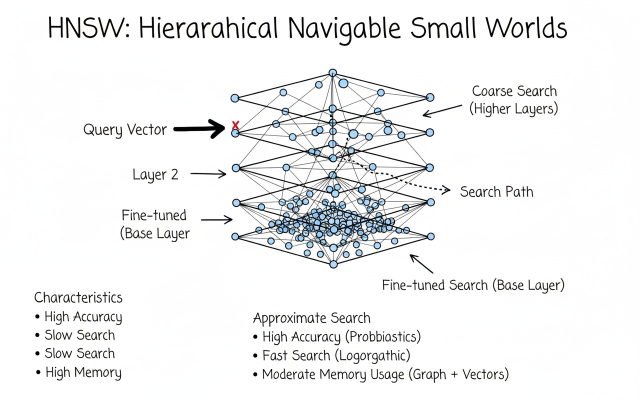
HNSW — IndexHNSWFlat
Hierarchical Navigable Small Worlds builds a multi-layer proximity graph. Querying means navigating neighbors rather than scanning all vectors.
Time: ~O(log N) (in practice)
Accuracy: tunable via efSearch
Memory: still stores full floats
index_hnsw = faiss.IndexHNSWFlat(128, 32)  # M=32 neighbors/node
index_hnsw.hnsw.efConstruction = 40
index_hnsw.hnsw.efSearch = 64
index_hnsw.add(Xn)              # add normalized vectors if using IP
D_h, I_h = index_hnsw.search(Qn, k=10)
Tuning heuristics
M (graph degree): 16–48 (more = better recall, more memory/build time)
efConstruction: 30–200 (higher = better graph quality)
efSearch: 32–256 (higher = better recall, slower queries)
Product Quantization (PQ) — IndexPQ
What is a PQ codebook?
PQ splits each vector into m equal chunks (subvectors). For each chunk, it learns k-means centroids (the codebook). Instead of storing floats, we store the centroid index for each chunk.
Storage per vector ≈
m × nbits / 8bytes
(e.g.,m=16,nbits=8→ 16 bytes per vector instead of128 × 4 = 512 bytes)Distance at query time uses precomputed lookup tables → very fast
Needs a training step to learn codebooks
d, m, nbits = 128, 16, 8   # m must divide d
index_pq = faiss.IndexPQ(d, m, nbits)
index_pq.train(X)          # learns codebooks via k-means
index_pq.add(X)            # stores codes, not floats
D_pq, I_pq = index_pq.search(Q, k=10)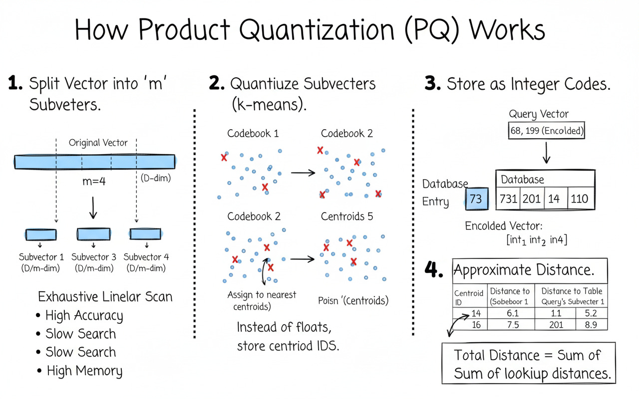
HNSW + PQ — IndexHNSWPQ
Now combine graph navigation (fast candidate search) with compressed vectors (tiny memory + fast lookups). This is a go-to setting for large, read-heavy workloads (RAG, semantic search, logs).
Speed: HNSW traversal + PQ distance lookups
Memory: much lower than HNSW-Flat
Accuracy: slightly lower than HNSW-Flat, tunable with
efSearch,m,nbits
m, nbits = 16, 8
index_hnsw_pq = faiss.IndexHNSWPQ(128, m, nbits)
index_hnsw_pq.hnsw.efConstruction = 40
index_hnsw_pq.hnsw.efSearch = 64
index_hnsw_pq.train(X)      # train codebooks
index_hnsw_pq.add(X)        # store compressed codes
D_hpq, I_hpq = index_hnsw_pq.search(Q, k=10)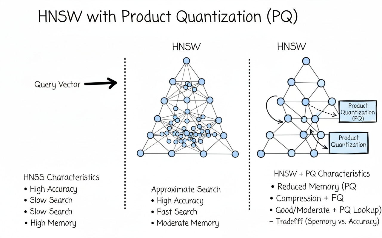
Trade-offs at a glance
Rule of thumb: if you’re memory-bound or at 10M+ vectors, HNSW+PQ is usually the sweet spot.

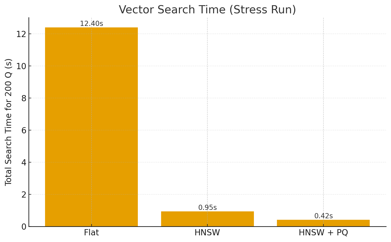
Benchmarks
I stress-tested three FAISS index types on a 24 GB RAM machine using ~20 GB worth of synthetic 384-dim embeddings.
Here’s the high-level view of how the benchmarks were calculated:
Index Build
Flat (Exact Search) → stored all vectors in float32.
HNSW → built a multi-layer graph with
M=32,efConstruction=40,efSearch=64.HNSW+PQ → trained PQ (
m=24,nbits=8) on a large sample, then built an HNSW graph over compressed codes.
Queries
200 random queries against the dataset.
For cosine similarity, vectors were L2-normalized and searched using Inner Product (IP).
Measured total query latency and average per query latency.
Metrics
Search Time: Wall-clock time to answer all 200 queries.
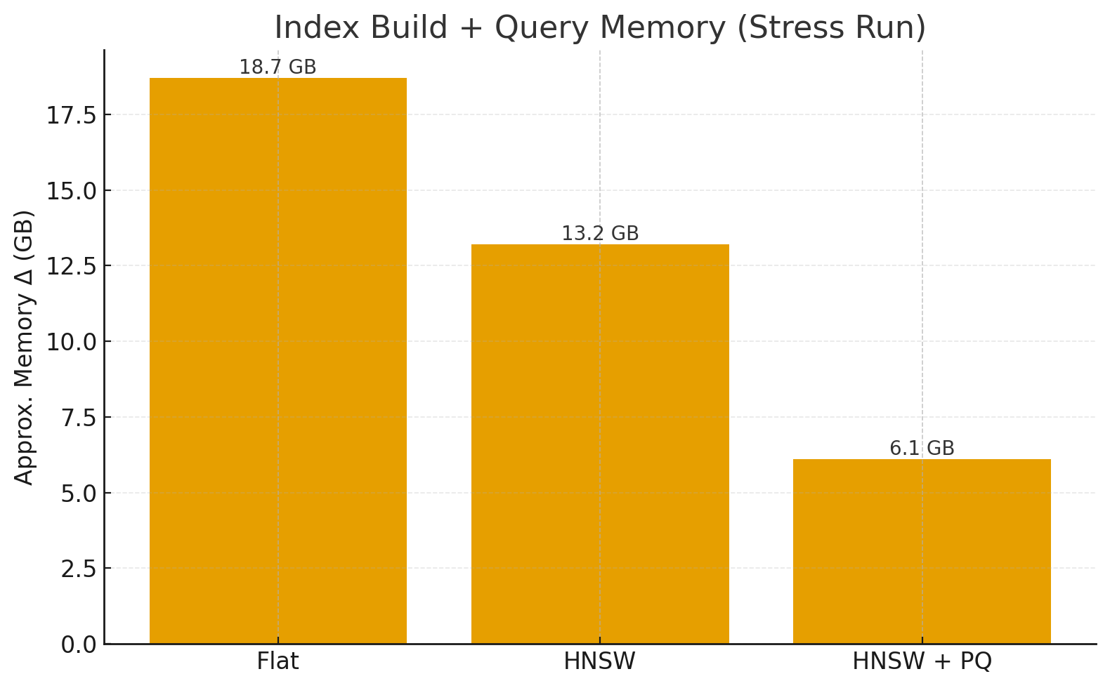
Memory Usage: ΔRAM observed during index build + queries (approx. process-level memory).
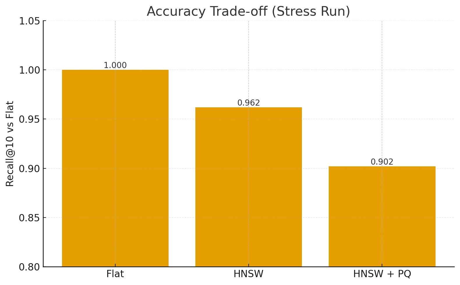
Recall@10: For each approximate method, overlap of retrieved neighbors vs. exact Flat search (gold standard).
Results (Stress Run)
IndexSearch Time (200Q)Memory Δ (GB)Recall@10Flat12.4 s18.7 GB1.000HNSW0.95 s13.2 GB0.962HNSW+PQ0.42 s6.1 GB0.902
🔑 Takeaways
Flat is exact but doesn’t scale (O(N)).
HNSW achieves ~10× faster queries with minimal recall loss.
HNSW+PQ further cuts memory and speeds up distance lookups, trading a bit more accuracy.
On a 24 GB machine, PQ allows fitting many more vectors while keeping queries sub-ms.